Volatility Modelling
This page was created to keep track of items related to volatility for personal reference. It may contain errors and should not be used as a substitute for any textbook or academic reference.
Definitions
- VIX9D: Nine day volatility
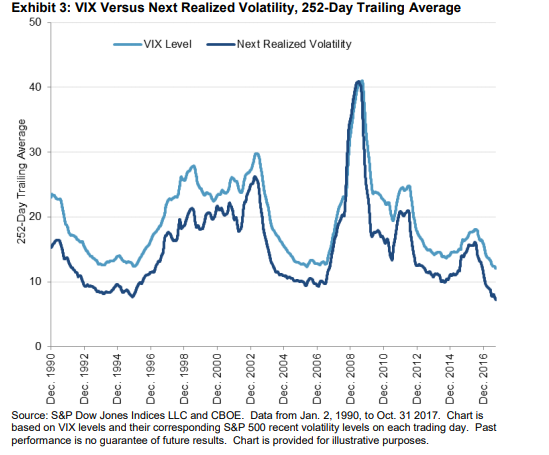
- VIX: The staple volatility index or 'fear gauge' for the economy. Measures the thirty-day implied volatility of options on the S&P500. The CBOE white paper contains the exact calculation if interested, but it essentially takes out-of-the-money (OTM) options outside of [23, 37] days to expiry and performs a weighted average of their implied volatility. The VIX often overstates the volatility that will be realized in 30-days, partly due to OTM puts being used for hedging strategies. The VIX is the square root of the risk-neutral expectation of the S&P 500 variance over the next 30 calendar days. It is the volatility of a variance swap, and not of a volatility swap.
- VIX3M: Three month volatility
- VIX6M: Six month volatility
- VIX1Y: One year volatility
Relationship between products:
VIX -> VIX Futures -> VIX Options -> VVIX
Realized volatility (RV): based on historical returns and is defined as the standard deviation of these returns for a given interval of time. This is an observation and does not depend on market participants expectations.
Implied volatility (IV): the level of volatility the market expects for the future, and the VIX purports to capture the 30-day version. It is not directly investable, but derivative products trade on it
Properties
Clustering/Persistence
It has been widely observed that volatility 'clusters'. In other words, small moves are often followed by small moves and large moves are often followed by large moves. This paper contains references to academic studies on the persistence (or memory) of changes in the VIX.
Mean Reverting
Historically, the VIX has reverted to a long term mean of around 13 (omitting tail events). Periods of extreme volatility create outliers which overstate where the VIX tends to revert to. This mean reversion property creates interesting trading strategies that allow market participants to bet that the VIX will revert once again.
Products
VIX Futures
In general, a futures contract is an obligation to buy or sell an asset at a predetermined price at some time in the future. In the case of VIX futures there is nothing to take possession of at the time of delivery, so cash is substituted.
Remember that the VIX does not track the actual (realized) volatility of the S&P500, it tracks the implied volatility of options on the S&P500 with a 30-day time to maturity (interpolated). A VIX futures contract is a forward contract on what 30-day IV will be on the expiration date. For example, on June 27 the VIX index was 34.73 and the July 22 VIX futures contract was 34.55. This means that if you purchase the contract at 34.55, you are betting that the VIX will be 34.55 or higher on July 22.
Fair value: Futures that can be hedged follow clear arbitrage-free pricing rules. If it’s cheaper to buy the underlying in the spot market and hold until maturity than it is to buy the future, then people will sell the future and long the underlying and pocket the difference (opposite applies as well). However, with VIX futures there is no underlying that can be purchased in a spot market to create this hedge, so the fair value is more difficult to determine. The VIX futures price reflects the markets best guess at where the VIX index will be at settlement and does not necessarily move in lockstep with the VIX spot price.
Since there is no cost of carry for VIX futures, the shape of the futures curve is only determined by expectations of future market vol. If vol is expected to increase in the future relative to now, the curve will be in contango. According to CBOE, 80% of all trading days have seen the second month contract higher than the front month.

Volatility Risk Premium: In general, implied volatility is greater than realized volatility. A reason for this is that investors are net long equities, volatility has traditionally been negatively correlated with asset prices, and so hedging your portfolio using volatility futures will come with a cost. Volatility sellers require compensation that is comparable to other asset classes (in expectation) otherwise they wouldn’t sell this protection. See the VXX description below to get a glimpse at the cost of owning volatility protection.
Below are two charts looking at VIX futures for the upcoming election period:


I see two main takeaways from the futures charts. The first is that the futures market is pricing in stock market volatility around the US election (Sept < Dec < Nov < Oct). The second is that the election volatility is nothing compared to what we experienced in March. Both results are intuitive (a planned election produces less uncertainty than a global pandemic), and it is helpful to reconcile our intuition with reality. Additionally, the futures are in contango through the election (before the November contract) and backwardation afterwards. I would argue this makes sense as well since we should expect the VIX to revert to its mean of approximately 13. This contango to backwardation structure also highlights the importance of looking at the VIX futures structure instead of spot VIX.
Exchange Traded Products on VIX Futures (VXX, VXZ, XIV [deceased])
Without going into details, VXX seeks to track short term VIX futures and owns the two front month VIX futures contracts to do so. Since the VIX futures term structure is usually in contango, the negative roll yield each month will cause VXX to tend to zero over time. The alternative explanation here is that since implied volatility is usually higher than realized, then it’s the convergence to spot price pulling both contracts down that causes the decrease in VXX rather than the cost of rolling contracts.
VXZ is similar to VXX but holds contracts 4-7 months out. Since the slope of the curve in contango is less steep the farther out you go, the negative roll yield will have less of an effect compared to VXX.
VIX Options
The Investopedia definition states that “a VIX option is a non-equity index option that uses the CBOE Volatility Index as its underlying asset”. I think this definition is misleading and relying on it would cause great confusion when looking at VIX option prices.
Since VIX options are based off VIX futures, the properties common to equity options do not necessarily hold. For example, say you were considering the following two SPY puts:
- A: Strike 300, September expiration
- B: Strike 300, October expiration
Without knowing the price of either put, we know that the price B > price A (assuming they both have bid/ask quotes showing). The time value inherent in B will guarantee that it will cost more than A.
However, if we try a similar exercise for VIX puts we can not come to the same conclusion. This is because a VIX put corresponds to the VIX future with the same expiration. The term structure of the VIX futures curve will help determine what direction this equality faces. If the curve is in contango, the September futures contract is lower than the October futures contract and so a September put could be worth more than an October put with the same strike.
Takeaway: In equity options, you can look at the spot price of the underlying to determine the price of the vanilla derivatives. For VIX options, you can’t look at the VIX spot price but instead need to look at the VIX futures curve to price the option.
VIX options are European style and cash settled. The options from which the VIX is calculated sum up to the square of the VIX. Because of this there is no way to statically replicate the VIX and so the Put-Call parity does not hold on VIX options.
See here for a CBOE fact sheet on the VIX, and here for a tool that plots the futures term structure.
Variance and Volatility Swaps
%matplotlib inline
import seaborn as sns
import main as vol
import warnings
sns.set()
warnings.filterwarnings('ignore')

df = vol.load_data()
vol.plot_timeseries(df)


The VIX is plotted from 1990 to present in the top left chart. In 2003 the CBOE changed its method of calculating the VIX, so I decided to separate the time series before and after that date. They used the new methodology on historical data, so it is fair to assume the 'old' time series exhibits the same properties as the current one. With this in mind I will treat the entire history as one homogeneous data set. Also notice that the clustering and mean-reverting properties discussed above are clearly visible (not to say this confirms they exist - just a visual aid).
In the top right there is the intraday high - low. In the most recent decade there appears to be larger and more frequent intraday moves in the VIX when compared with the previous decade. My speculation is this is due to increased high frequency trading, information disseminating more quickly throughout the financial markets, or potentially the switch to weekly SPX options in 2014. Analysis would be needed to determine if any of the above points are contributing factors, or if the observed spikes are more noise than signal.
It's always helpful to visualize the data we are working with, so let's look at a few boxplots for the VIX:
vol.grp_plot(df)


The boxplot for the day of the week shows no noticeable trend, which makes sense. The monthly view shows summer months as less slightly less volatile than other months, with the last two crises clearly visible in March (2020) and October/November (2008). Finally the yearly view shows most years are relatively calm with a few volatile days and highlights just how pronounced 2008 and 2020 were in terms of market volatility.
While the VVIX is not the center of attention on this page, it is interesting to look at its plots as well:
vol.grp_plot(df,col='VVIX Close')


With the caveat that there is significantly less VVIX data than there is VIX data, it appears that the VVIX has been increasing on average since 2008. I do not have any intuition for the cause of this, but interpreted literally it would seem there is more uncertainty on the expected value of the VIX. Potentially the recent memory of the GFC has caused participants to use different hedging products such as VIX futures, creating more implied volatility due to the demand.
Above it was stated that volatility clusters, but how do we test for this in a set of data?
One way is to see if there is strong auto-correlation at different lags. If there is, it suggests that a recent move has predictive power for subsequent moves.
vol.plot_auto_corr(df)


Mean Component: The first chart above shows that recent moves in the VIX have little predictive power in the future return of the VIX.
Variance Component: However the second chart shows that the squared log-return has significant predictive power (note the difference in the y-axis). This supports the property that volatility clusters: small moves are followed by small moves (positive or negative), similarly for large moves.
Models
Model 1: Ornstein-Uhlenbeck with constant variance
https://en.wikipedia.org/wiki/Ornstein%E2%80%93Uhlenbeck_process
$dX_t = \theta(\mu - X_t)dt + \sigma dW_t$
with $\theta > 0$ and $\sigma > 0$
In English, the model says that process $X$ (which will be the VIX in our case) will revert to its mean $\mu$ over time. The parameter $\theta$ affects how quickly the process reverts to its mean. Additionally, there is some random noise ($X_t$) associated with the process, and it scales with $\sigma$.
In order to simulate paths, I used Euler discretization for simplicity:
$X_t = X_{t-1} + \theta(\mu - X_{t-1})\Delta_t + \sigma \sqrt{\Delta_t}Z_t$
Where $Z_t$ is a standard normal random variable
static_vix = vol.single_OU(df)  # MR simulation
vol.plot_sims(df, static_vix, num_plots=3)

Pros:
- Looking at the line chart, the process appears to be mean reverting (as specified in our model).
Cons:
- Negative values. To remedy this we could take the absolute value of the process after each change, we could work in log-prices.
- Looking at the histogram, we can see the VIX has positive skew whereas our model has little to no skew and fails to go far out in the distribution.
- The mean reversion process is much faster with the VIX than with our model, but only after extremely large jumps (i.e a constant theta value does not seem realistic for big jumps).
- Variance was assumed constant but in reality vol-of-vol is not constant (i.e the VVIX exists).
Below some summary statistics are computed to compare the simulations. Fisher kurtosis is computed, so kurtosis = 0 is Normal.
You can clearly see that despite the mean and standard deviation being on target, the skew and kurtosis are nowhere close.
vol.compare_stats(df, static_vix, sim_name='Static VIX')
Model 2: Double Ornstein-Uhlenbeck model
$\sigma$ in our original model is certainly not constant (think of any financial event, minor or major), and so we should let it wander around as well
$dX_t = \theta_1(\mu_1 - X_t)dt + \sqrt{V_t} dW_t^1$
$dV_t = \theta_2(\mu_2 - V_t)dt + \sigma dW_t^2$
Where $W_t^1$ and $W_t^2$ are correlated using the correlation between the VIX and VVIX.
Again the process will be simulated using Euler discretization. Additionally the process will be reflected off the x-axis to avoid negative values.
dynamic_vix, static_vvix = vol.double_OU(df)  # MR simulation
vol.plot_sims(df, dynamic_vix, num_plots=3)
vol.compare_stats(df, dynamic_vix, sim_name='Dynamic VIX')

The chart and statistics look similar to before, suggesting that the model may not be sufficient to explain the tails of the VIX. Introducing jumps or regime switching may be necessary.
Since we have the VVIX modeled now as well, I have plotted it below. In order to calibrate the model I simulated it for the same period as the VIX even though it was created much later.
vol.plot_sims(df, static_vvix, num_plots=3, col_name='VVIX Close')
vol.compare_stats(df, static_vvix, sim_name='Static VVIX', col_name='VVIX Close')

The VVIX model suffers the same issue of being unable to match the skew and kurtosis of the true VVIX.
Model 3: Jump Process
To this point we have been suffering from low skew and negative kurtosis, whereas the VIX has been seen to be positively skewed with positive excess kurtosis. Adding jumps to our model should help thicken the tail of our histogram.
Additionally, $\theta$ is being changed as well. Whereas it was fixed at 1/2 before, it now takes on a value of 2 for values below 10. This was added as the VIX has consistently met extremely strong resistance as it approaches nine, and so our model should reflect that.
$X_t = X_{t-1} + \theta(\mu - X_{t-1})\Delta_t + \sigma \sqrt{\Delta_t}Z_t + X_{t-1}*|J_t|*Q_t$
$Q_t$ takes on a value of 0 or 1 at each time step, drawn from a poisson process.
$|J_t|$ is the absolute value of the normally distributed jump size. I included the absolute value as the mean-reverting nature of the VIX will allow it to come back down from outsized jumps up. Adding jumps down is a desirable feature, but requires recent memory in the model to only jump down after significant jumps up.
This is a poorly behaved process. Since there is no guarantee that jumps will not follow each other, multiplying by a scalar multiple could cause the process to jump very quickly in a few time steps (albeit with low probability). Finding the distribution of jumps and their persistence is an important next step for a calibrated jump process.
jump_vix = vol.jump_mean_reverting(df)  # MR simulation
vol.plot_sims(df, jump_vix, num_plots=3)
vol.compare_stats(df, jump_vix, sim_name='Jump VIX')

As we can see above, adding jumps can significantly increase the skewness and kurtosis of our distribution.
The next section to be added will be on GARCH models, which will help explore persistence in changes in the VIX.